Dead Neurons
Table of contents
- Peeking inside a hidden layer
- But how can we decide which number to multiply? (Initialization)
- Summary
I implemented some techniques used in a research paper for n-gram language modeling. It is a simple MLP-based trigram language model that takes three characters’ tokens as input, passes them into an embedding layer, then a hidden linear layer, and finally predicts the next character’s token.
Here are the hyperparameters I used:
n = 3 #trigram model
emb_sz = 2 #latent factor
n_hidden = 100
vocab_sz = len(chars) # it's 27
Here is the architecture:
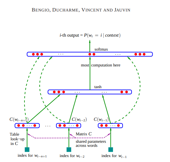
Source: https://www.jmlr.org/papers/volume3/bengio03a/bengio03a.pdf
C = torch.randn(vocab_sz, emb_sz)
w1 = torch.randn(n*emb_sz, n_hidden)
b1 = torch.randn(n_hidden)
w2 = torch.randn(n_hidden, vocab_sz)
b2 = torch.randn(vocab_sz)
# Setting up gradient requirements
parameters = [C, w1, b1, w2, b2]
for p in parameters:
p.requires_grad = True
# ---------------------------------------------------
# training
epoch = 200_000
bs = 32 # batch sz
for i in range(epoch):
# mini batch
idx = torch.randint(0, xtrain.shape[0], size=(bs,))
xbs, ybs = xtrain[idx], ytrain[idx] # batch
# forward pass
emb = C[xbs]
hpreact = emb.view(emb.shape[0], -1) @ w1 + b1
h = torch.tanh(hpreact)
logits = h @ w2 + b2
loss = F.cross_entropy(logits, ybs)
perplexity = torch.exp(loss)
# backward pass
for p in parameters:
p.grad = None
loss.backward()
# update
lr = 0.01 if i < 100_000 else 0.001
for p in parameters:
p.data -= p.grad.data * lr
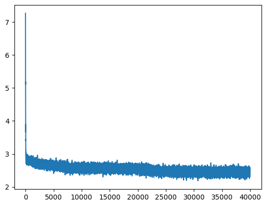
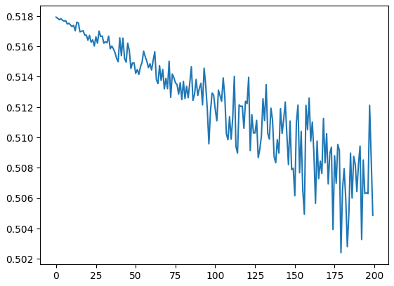
# track
lossi.append(loss.log10().item())
if i%10000 == 0:
print(f"epoch: {i:7d}/{epoch:7d} | loss: {loss.item():.4f} | perplexity: {perplexity.item():.4f}")
epoch:       0/    200 | loss: 9.9113 | perplexity: 20157.0859
epoch:      10/    200 | loss: 4.8961 | perplexity: 133.7642
epoch:      20/    200 | loss: 3.5018 | perplexity: 33.1759
epoch:      30/    200 | loss: 3.0638 | perplexity: 21.4093
epoch:      40/    200 | loss: 2.8681 | perplexity: 17.6032
epoch:      50/    200 | loss: 2.8150 | perplexity: 16.6932
Firstly, I want to explain why we need to initialize the weights of our model with good values. As observed, the initial loss is very high, and then subsequent losses are very low. The weights we initialized are significantly incorrect, as some are very confidently wrong while others can be overly confident. This necessitates spending time and computational resources to correct them before starting unbiased learning. Thus, improving parameter initialization can help us skip this unnecessary step, which otherwise wastes energy and computation.
Let’s visualize the logits in a histogram:
plt.hist(logits.tolist(), 50);
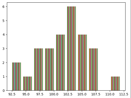
The mean is near 100 or so. We can achieve our objectives if the logits obtained in the final layer are low instead of very high. To accomplish this, we can initialize the bias of the final layer to zero, allowing the neural network to learn how to offset it by itself, and initialize the weights with small numbers.
C  = torch.randn(vocab_sz, emb_sz)
w1 = torch.randn(n*emb_sz, n_hidden)
b1 = torch.randn(n_hidden)
w2 = torch.randn(n_hidden, vocab_sz) * 0.01
b2 = torch.randn(vocab_sz) * 0
plt.hist(logits[0].tolist(), 50);
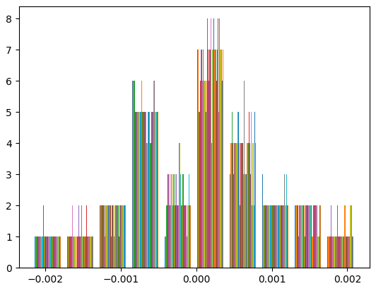
We should not initialize weights with zero, just as the bias, because this would cause all neurons to update in the same way, resulting in symmetric and redundant weights throughout the training process.
Peeking inside a hidden layer
The second issue I want to address concerns the hidden layer. Consider the forward pass
idx = torch.randint(0, xtrain.shape[0], size=(bs,))
emb = C[xtrain[idx]]
embinp = emb.view(emb.shape[0], -1)
h = torch.tanh(embinp @ w1 + b1)
logits = h @ w2 + b2
loss = F.cross_entropy(logits, ytrain[idx])
In this code snippet, bs represents the batch size, C is the embedding matrix, h is the output of the hidden layer (shaped BSxN_hidden), and w1, b1, w2, b2 are the linear layer’s weights and biases, with cross-entropy loss calculated at the end. Refresher: cross-entropy loss involves calculating the softmax of logits and then calculating its log likelihood, commonly used as a loss function in classification tasks. Everything seems fine, but if we examine the hidden layer’s numbers, something is amiss. Here’s the training loss:
epoch:     0/ 200000 | loss: 2.7297 | perplexity: 15.3288
epoch: 10000/ 200000 | loss: 2.5840 | perplexity: 13.2500
Perplexity, is the exponential of cross-entropy loss (
loss.exp()). The exponential of loss, which changes with very few points, is much easier to understand when spread using exponential.
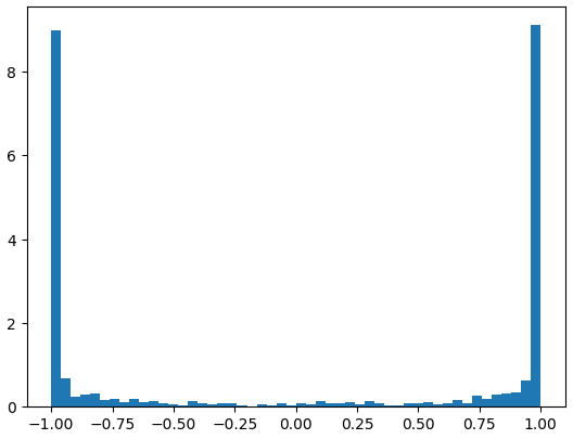
A deeper problem lurks within this neural net and its initialization. To visualize this, let’s flatten the hidden layer (h) and plot it in a histogram. We observe that most numbers lie near 1 and -1 instead of in between, which occurs because tanh is a squashing function that compresses everything into its flat region at 1 or -1. This means that these neurons are either highly active or highly inactive. As Andrej Karpathy pointed out, “if you’re not very experienced with gradient descent, you might think this is okay, but if you are experienced with the black magic of gradient descent, then you might be sweating already”.
>>>h

tensor([[-1.0000,  0.9997, -1.0000,  ...,  1.0000, -1.0000,  0.2273],
        [ 0.3959,  0.9912, -1.0000,  ..., -0.9820,  0.6797, -0.9998],
        [ 0.8695, -0.9592, -0.4954,  ...,  0.4124, -0.8499,  0.9920],
        ...,
        [ 0.9987,  0.9952, -0.9996,  ...,  0.8290, -0.9994, -1.0000],
        [-0.9993,  0.9991, -1.0000,  ..., -0.6726, -1.0000,  1.0000],
        [ 0.9954, -0.2170, -1.0000,  ..., -0.9923,  0.0163, -0.8219]],
Most of them are near 1 and -1.
plt.hist(h.view(-1).tolist(), 50);
We can actually do the same small number multiplication to the W1 and B1 which gives us hidden state (h).
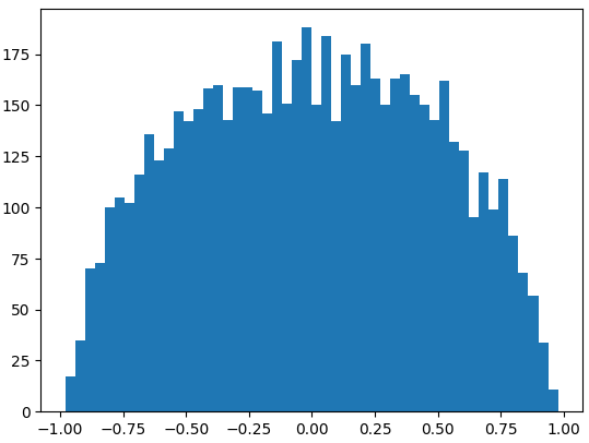
We can mitigate this issue by applying the same small number multiplication to W1 and B1, which produces a more desirable hidden state (h).
w1 = torch.randn(n*emb_sz, n_hidden) * 0.1
b1 = torch.randn(n_hidden) * 0.01

#later
plt.hist(h.view(-1).tolist(), 50);
This is because, as we can observe, the differentiation of tanh is as follows:
x = data
t = (math.exp(2*x) - 1)/(math.exp(2*x) + 1)
out = t

# backward
grad = (1 - t**2) * out.grad
Regardless of whether we increase or decrease the input data to the tanh function, 1 - t^2 would be zero, resulting in zero gradients. Notice that the gradients always decrease. If the weight initialization is poor and all data points lie above 1 or below -1, they will all be squashed into the flat region of 1 and -1. Consequently, the gradients will be destroyed. To further illustrate this, let’s visualize our hidden layer using matplotlib.
We take the absolute value of each value and observe how frequently they are fully activated.
plt.figure(figsize=(16,16))
plt.imshow((h.abs()<0.99).tolist(), cmap='gray')
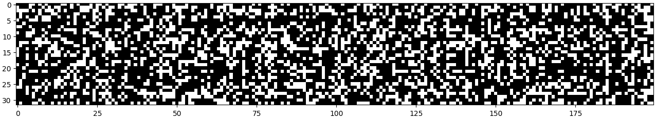
In this plot, white cells indicate dead neurons. If a complete column is white, it will completely destroy any gradients flowing through it, and weights beyond that column will never learn because they will never receive gradients.
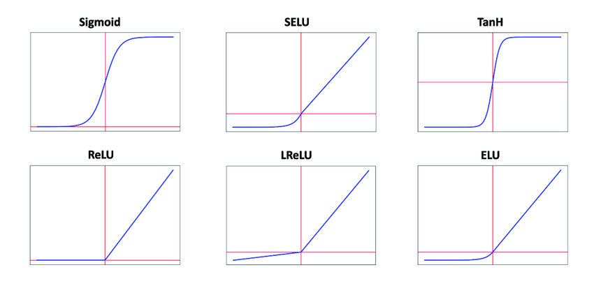
Similar issues occur with other activation functions, such as Sigmoid, Relu, and ELU, because they also have a squashing plane. A research paper (https://arxiv.org/pdf/1502.01852.pdf) extensively studied this phenomenon, particularly in the context of Relu and PRelu in convolutional neural nets. They found that if a Relu neuron never activates for any input in the dataset, its weights and biases will never receive gradients, rendering it ineffective. Conversely, if it receives excessively large gradients (possible with high learning rates), it will be knocked out of the data manifold, preventing it from learning from the rest of the training data.
They also proposed a solution to this problem: when initializing weights and biases in a Gaussian distribution, if the resulting standard deviation shifts too much, we need to retain the original standard deviation. We can achieve this by multiplying the weight matrix by a small number during initialization. Surprisingly, the number we multiply is the new standard deviation for that matrix.
X1 = torch.randn(1000,100)
>>> X2 = torch.randn(100,1000)

>>> X1.mean(), X1.std()
(tensor(-0.0070), tensor(1.0002))

>>> X2.mean(), X2.std()
(tensor(-0.0032), tensor(1.0020))

>>> (X1@X2).mean()
tensor(-0.0096)
>>> (X1@X2).std()
tensor(10.0116)

>>> X2 = torch.randn(100,1000) * 0.2
>>> (X1@X2).mean()
tensor(0.0020)
>>> (X1@X2).std()
tensor(2.0032)
So, the standard deviation of the matrix changes based on the number we multiply.
But how can we decide which number to multiply?
It turns out there’s a mathematical principle. For example, in Relu, half of the data is discarded to 0 for any input in the dataset. We can then amplify the remaining half of the data with a gain. Most researchers currently use the square root of the fan-in to multiply with the weights (as mentioned above). The fan-in represents the input features of a layer.
w1 = torch.randn(n*emb_sz, n_hidden) * (n*emb_sz)**0.5
b1 = torch.randn(n_hidden)

# for w1: n*emb_sz is fan-in (feature in)
# x**0.5 is handy for calculating the square root
Another popular initialization method is Kaiming initialization, based on the same theory, but with different gains for each activation function. Here is a link to the documentation: https://pytorch.org/docs/stable/nn.init.html#torch.nn.init.kaiming_normal_
PyTorch calculates the gain as follows: https://pytorch.org/docs/stable/nn.init.html#torch.nn.init.calculate_gain
A gain might be necessary because activation functions like Relu and Tanh squash the input. Researchers today typically use the square root of the fan-in to multiply with the weights, as demonstrated above. Because there are other normalization techniques such as batch normalization. instance normalization, layer normalization, group normalization and stronger optimization algorithms besides stochastic gradient descent, such as RMS Prop and Adam.
Summary
The activation function squashes the weights, so we should be concerned about how we initialize them. For example, in the tanh function, we don’t want them to saturate to one or negative one. To maintain good performance, we normalize them with a gain, which can typically be found as the square root of the fan-in. There are additional mathematical principles to consider, such as the Kaiming initialization, which also utilizes a gain multiplied by a constant for different activations like Sigmoid, Linear, and ReLU.