Batch Normalization
Table of contents
Understanding why training deep neural networks can be fragile is crucial. Issues like dead neurons or saturation of non-linearity, and the vanishing or exploding gradients have caused problem for deep learning for years. However, there’s a beacon of hope that emerged around 2015: Batch Normalization.
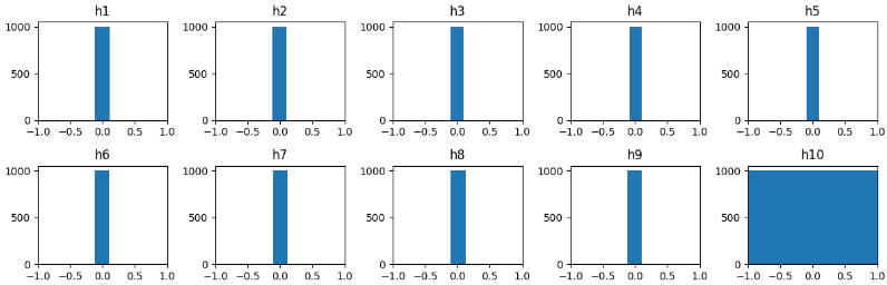
Here is a visualization of problem using graph. Say we have 1000 datapoints and each has 500 embeddings (latent factors).
D = torch.randn(1000, 500)
Y = torch.randn(1000, 1) * 0.1
And we have 10 layers each with 500 * 500 neurons.
l1 = Linear(500, 500)
l2 = Linear(500, 500)
l3 = Linear(500, 500)
l4 = Linear(500, 500)
l5 = Linear(500, 500)
l6 = Linear(500, 500)
l7 = Linear(500, 500)
l8 = Linear(500, 500)
l9 = Linear(500, 500)
l10 = Linear(500, 1)
And we train it.
  ...
  h1 = l1(D)
  h1 = h1.tanh()
  h2 = l2(h1)
  h2 = h2.tanh()
  ...
  h10 = l10(h9)
  h10 = h10.tanh()
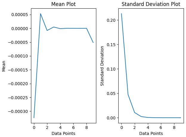
If we see the statistics of hidden layer’s activations, h1, h2, the standard deviation of the layer is getting close to one. Standard deviation is the distance between the mean and data point, which implies that the data is shrinking closer and closer to mean.
And that’s what happens exactly:
H0 -> mean: -0.0003, std:  0.2132
H1 -> mean:  0.0001, std:  0.0476
H2 -> mean: -0.0000, std:  0.0106
H3 -> mean:  0.0000, std:  0.0024
H4 -> mean: -0.0000, std:  0.0005
H5 -> mean:  0.0000, std:  0.0001
H6 -> mean:  0.0000, std:  0.0000
H7 -> mean: -0.0000, std:  0.0000
H8 -> mean:  0.0000, std:  0.0000
H9 -> mean: -0.0001, std:  0.0000
The Batch Normalization paper marked a significant milestone in deep learning. It was the first normalization layer technique to tackle the fragility of deep neural net training. Released by the Google team, specifically Google DeepMind, this technique provided a groundbreaking solution to the problem of activation saturation in weights initialization.
As shown above in a tanh activation: if the weights are too large, activations saturate at 1 and -1, and if they’re too close to zero, they saturate in the middle. Neither scenario is ideal.
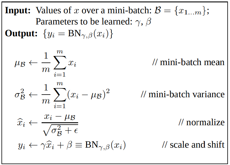
Batch Normalization paper is the first normalization layer technique that is used in deep learning. It addressed the problem of activations saturation in the weights that we initialize. We want the weights to be roughly Gaussian. The basic idea of this paper was “if we want the activation of the hidden state to be Gaussian, then why don’t we take that activation and normalize them to be Gaussian”. Sounds funny but it actually works, we take the mean and standard deviation of the hidden state activations and we subtract the mean from each data point and divide them with standard deviation normalizes them to be roughly Gaussian.
# if "h2" is the activation of hidden layer "l2", then
  h2 = l2(h1) # get the acts
  bx = b1(h2) # pass them to batchNorm layer
  h2 = h2.tanh() # non-linearity

  # The paper formula looks like
  xbs # mini batch
  xmean = xbs.mean(1, keepdim=True) # batch mean
  xvar = xbs.var(1, keepdim=True)   # batch var
  h_normalized = (h2 - xmean) / (xvar + epsilon)**0.5
But this will take away the flexibilty of weight and it will never learn, to fix this we take this normalized hidden state and multiply them with learnable weights (called Gamma) and add bias called beta, This gives neural net the full ability to learn the new data points. The gain amplifies (visualize vertically in an x/y plane for understanding) and bias helps the neural net as an offset (visualize horizontally, as when we add something to a number it shiftes to-and-forth the number line).
# initialization of Gamma and beta
gamma = torch.ones(hidden_sz)
beta = torch.zeros(hidden_sz)

gamma * h_normalized + beta # similar to XW + B :)

The problem of activation for large neural net will become very quickly intractable to keep activation of hidden Layer roughly Gaussian as to keep them unsaturated. But sprinkling multiple batch mobilization layer is easy and effective but the comes with a terrible cost.
The training the neural net with mini-batch, we did that for efficiency and training fast and parallelly. But in BatchNorm, we are again COUPLING each data points in batches in the forward and backward pass. Each logits is not just a function of previous hidden layer, but also the function of the data point that came in that particular Batch. To understand this, if we react for any one of those input example it is going to change slightly depending upon what the other input is in those batch. So, H will also change because it will be impacted by H-mean and H-Standard Deviation. It will slightly jitter the edge depending upon the value of mean and standard deviation.
TLDR: As the mean and var are calculated along the dimension, this means we are again coupling the datapoint. So any changes in any one of the input in a batch will jitter the activation of the batchnorm layer.
We could think that this is a bug, but it’s actually good for training and neural net because it acts as a regularizer and kinda adds noise to the input data and sensitivity to weight initialization. It prevents overfitting and also helps to generalize (it jitters the input data. Because each input data is subtracted by mean and then divided by standard deviation calculated across the batch for each data point).
It works so well. which made it hard to move on to different techniques because no one likes the property of coupling batches but it is the first Normalization layer technique. It has regularization effect, stable training. It worked quite well. Because of The regularization effect.
Strange output of coupling
Let’s say we trained a model and we want to deploy how can we do that if in the forward pass expects a mean and standard deviation of batch? That means it expects a batch as an input and not a data point. So the authors of the research paper proposed this solution:
Option 1.
Calibrate mean and standard deviation of training data after training as an additional step (between training and validation)
Option 2.
Keep track of standard deviation and mean in a variable in the training Loop. (called Running variable)
running_mean = 0.999 * running_mean + 0.001 * xmean
running_std = 0.999 * running_std + 0.001 * xstd
Note: There is a epsilon. In the paper and we add that epsilon when we calculate the standard deviation. We add that epsilon to variance, in the denominator. To add stability/safety in the calculation.
Second note: We don’t need bias for the layer before a batch normalization layer. Because in the next step we take the mean of the activations and subtract it. It basically cancels out. The bias is useless. This don’t break anything but just waste of computation. Because it never take parts in gradients. So whenever in a neural net if you are using batch normalization, in the layer prior to batch normalization layer we set the bias to False.
Here is the full implementation of multi layer neural net with batch normalization layer:
class Linear:
  def __init__(self, fan_in, fan_out, bias=True):
    self.weight = torch.randn((fan_in, fan_out)) * 0.1 # / fan_in**0.5 # note: kaiming init
    self.bias = torch.zeros(fan_out) if bias else None
  def __call__(self, x):
    self.out = x @ self.weight
    if self.bias is not None:
      self.out += self.bias
    return self.out

  def parameters(self):
    return [self.weight] + ([] if self.bias is None else [self.bias])

class BatchNorm1d:
  def __init__(self, dim, momentum=0.1, eps=1e-5):
    self.training = True
    self.eps = eps
    self.momentum = momentum
    self.gamma = torch.ones(dim)
    self.beta = torch.zeros(dim)
    self.running_mean = torch.zeros(dim)
    self.running_var = torch.ones(dim)

  def __call__(self, x):
    if self.training:
      if x.ndim == 2:
        dim = 0
      elif x.ndim == 3:
        dim = (0,1)
      xmean = x.mean(dim, keepdim=True)
      xvar = x.var(dim, unbiased=True, keepdim=True)  #Notice: unbiased=True
      # In statistics, Bessel's correction is the use of n − 1 instead of n in the formula for the sample variance and sample standard deviation
    else:
      xmean = self.running_mean
      xvar = self.running_var
    dx = (x - xmean)/torch.sqrt(xvar + self.eps)
    self.out = self.gamma * dx + self.beta

    if self.training:
      with torch.no_grad():
        self.running_mean = (1.0 - self.momentum) * self.running_mean + self.momentum * xmean
        self.running_var = (1.0 - self.momentum) * self.running_var + self.momentum * xvar
    return self.out

  def parameters(self):
    return [self.gamma, self.beta]

class Tanh:
  def __call__(self, x):
    self.out = torch.tanh(x)
    return self.out
  def parameters(self):
    return []
# Hyperparameters
n = 3 # trigram model
emb_sz = 10
n_hidden = 100
vocab_sz = len(chars) # it's 27

# -----------------------------------------------
C = torch.randn(vocab_sz, emb_sz, generator=g)
layers = [
  Linear(emb_sz*n, n_hidden, bias=False), BatchNorm1d(n_hidden), Tanh(),
  Linear(n_hidden, n_hidden, bias=False), BatchNorm1d(n_hidden), Tanh(),
  Linear(n_hidden, n_hidden, bias=False), BatchNorm1d(n_hidden), Tanh(),
  Linear(n_hidden, n_hidden, bias=False), BatchNorm1d(n_hidden), Tanh(),
  Linear(n_hidden, n_hidden, bias=False), BatchNorm1d(n_hidden), Tanh(),
  Linear(n_hidden, vocab_sz, bias=False), BatchNorm1d(vocab_sz)
]
# -----------------------------------------------

with torch.no_grad():
  layers[-1].gamma *= 0.1
  for l in layers[:-1]:
    if isinstance(l, Linear):
      l.w *= 1.0

parameters = [C] + [p for l in layers for p in l.parameters()]
print(sum(p.nelement() for p in parameters))

for p in parameters:
  p.requires_grad = True
Training log:
epoch       0/20000   |   loss: 3.3056   |   perx: 27.2652
epoch     100/20000   |   loss: 3.2400   |   perx: 25.5348
epoch     200/20000   |   loss: 3.1552   |   perx: 23.4585
epoch     300/20000   |   loss: 3.1343   |   perx: 22.9729
epoch     400/20000   |   loss: 2.9765   |   perx: 19.6192
epoch     500/20000   |   loss: 3.0426   |   perx: 20.9598
epoch     600/20000   |   loss: 2.9243   |   perx: 18.6212
epoch     700/20000   |   loss: 2.9431   |   perx: 18.9746
epoch     800/20000   |   loss: 2.7778   |   perx: 16.0831
epoch     900/20000   |   loss: 2.7860   |   perx: 16.2167
epoch    1000/20000   |   loss: 2.7030   |   perx: 14.9249
epoch    1100/20000   |   loss: 2.8019   |   perx: 16.4762
epoch    1200/20000   |   loss: 2.7259   |   perx: 15.2699
epoch    1300/20000   |   loss: 2.7281   |   perx: 15.3041
epoch    1400/20000   |   loss: 2.6197   |   perx: 13.7310
epoch    1500/20000   |   loss: 2.6625   |   perx: 14.3316
epoch    1600/20000   |   loss: 2.6108   |   perx: 13.6103
epoch    1700/20000   |   loss: 2.7052   |   perx: 14.9580
epoch    1800/20000   |   loss: 2.6034   |   perx: 13.5096
epoch    1900/20000   |   loss: 2.5848   |   perx: 13.2610
epoch    2000/20000   |   loss: 2.1021   |   perx: 8.1833
Source
- Inspired from this lecture.
- Complete implementation: github link