Understanding loss.backward()

Relying on any library is not good; therefore, this time, removing this black box and understand what’s happening inside. Writing a backward pass manually would be helpful. Backpropagation is not something that works magically or automatically if you are hoping to debug. In other words, it is easy to fall into the trap of abstracting away the learning process, believing that you can simply stack arbitrary layers together and backprop will magically make them work on your data. So let’s look at a few explicit examples where this is not the case in quite unintuitive ways.

This blog post is clearly set of personal notes for the notes by Andrej Karpathy’s cs231n lectures.¹²³

Simple expressions and interpretation of the gradient
Compound Expressions with Chain Rule
Intutive understanding of backpropogation
Backprop in practice: Staged computation
Gradients for vectorized operations
Gradient checking
Sources

Simple expressions and interpretation of the gradient

Let's start with simple expressions to develop the notation and conventions for more complex ones. Consider a straightforward multiplication function of two numbers \( f(x,y) = xy \). It's a matter of simple calculus to derive the partial derivative for either input: \[ \frac{\partial f}{\partial x} = y \quad \text{and} \quad \frac{\partial f}{\partial y} = x \] Interpretation: Derivatives indicate the rate of change of a function with respect to that variable around an infinitesimally small region near a particular point: \[ \frac{df(x)}{dx} = \lim_{h \to 0} \frac{f(x+h) - f(x)}{h} \] A technical note is that the division sign on the left-hand side is not a division; it indicates that the operator \( \frac{d}{dx} \) is being applied to the function \( f \), returning a different function (the derivative). When \( h \) is very small, the function is well-approximated by a straight line, and the derivative is its slope. In other words, the derivative on each variable tells you the sensitivity of the whole expression to its value. For example, if \( x = 4, y = -3 \), then \( f(x,y) = -12 \) and the derivative on \( x \), \( \frac{\partial f}{\partial x} = -3 \), indicates that increasing the value of \( x \) by a tiny amount would decrease the whole expression by three times that amount. Similarly, since \( \frac{\partial f}{\partial y} = 4 \), increasing \( y \) by a small amount would increase the output of the function by four times that amount.

The Gradient: The gradient \( \nabla f \) is the vector of partial derivatives, so we have \( \nabla f = [\frac{\partial f}{\partial x}, \frac{\partial f}{\partial y}] = [y, x] \). Though technically a vector, we'll often use terms like "the gradient on \( x \)" instead of the technically correct phrase "the partial derivative on \( x \)" for simplicity. We can also derive the derivatives for the addition operation: \[ f(x,y) = x+y \quad \rightarrow \quad \frac{\partial f}{\partial x} = 1 \quad \text{and} \quad \frac{\partial f}{\partial y} = 1 \] That is, the derivative on both \( x \) and \( y \) is one, regardless of their values. This makes sense since increasing either \( x \) or \( y \) would increase the output of \( f \), and the rate of increase would be independent of their actual values. Let's consider the max operation: \[ f(x,y) = \max(x,y) \quad \rightarrow \quad \frac{\partial f}{\partial x} = \begin{cases} 1 & \text{if } x \geq y \\ 0 & \text{otherwise} \end{cases} \quad \text{and} \quad \frac{\partial f}{\partial y} = \begin{cases} 0 & \text{if } x \geq y \\ 1 & \text{otherwise} \end{cases} \] Here, the (sub)gradient is 1 on the input that was larger and 0 on the other input. Intuitively, if \( x = 4 \) and \( y = 2 \), then the max is 4, and the function is not sensitive to the setting of \( y \). That is, if we were to increase it by a tiny amount \( h \), the function would keep outputting 4, and therefore the gradient is zero—there's no effect. Of course, if we were to change \( y \) by a large amount (e.g., larger than 2), then the value of \( f \) would change, but the derivatives tell us nothing about the effect of such large changes on the inputs of a function; they are only informative for tiny, infinitesimally small changes, as indicated by the \( \lim_{h \to 0} \) in their definition.

Compound Expressions with Chain Rule

Let's now consider more complicated expressions that involve multiple composed functions, such as \( f(x,y,z) = (x+y)z \). While this expression is simple enough to differentiate directly, we'll take a particular approach that will be helpful for understanding the intuition behind backpropagation. Specifically, note that this expression can be broken down into two expressions: \( q = x+y \) and \( f = qz \). Moreover, we know how to compute the derivatives of both expressions separately, as seen in the previous section. \( f \) is just the multiplication of \( q \) and \( z \), so \( \frac{\partial f}{\partial q} = z \), \( \frac{\partial f}{\partial z} = q \), and \( q \) is the addition of \( x \) and \( y \) so \( \frac{\partial q}{\partial x} = 1 \), \( \frac{\partial q}{\partial y} = 1 \). However, we don’t necessarily care about the gradient on the intermediate value \( q \)—the value of \( \frac{\partial f}{\partial q} \) is not useful. Instead, we are ultimately interested in the gradient of \( f \) with respect to its inputs \( x, y, z \). The chain rule tells us that the correct way to "chain" these gradient expressions together is through multiplication. For example, \( \frac{\partial f}{\partial x} = \frac{\partial f}{\partial q} \frac{\partial q}{\partial x} \). In practice, this is simply a multiplication of the two numbers that hold the two gradients. Let's see this with an example:

# inputs
x = -2; y = 5; z = -4

# forward pass
q = x + y  # q becomes 3
f = q * z  # f becomes -12

# backward pass (backpropagation) in reverse order:
# First backprop through f = q * z
dfdz = q  # df/dz = q, so gradient on z becomes 3
dfdq = z  # df/dq = z, so gradient on q becomes -4
dqdx = 1.0
dqdy = 1.0
# Now backprop through q = x + y
dfdx = dfdq * dqdx  # The multiplication here is the chain rule!
dfdy = dfdq * dqdy

We are left with the gradient in the variables \([ \frac{\partial f}{\partial x}, \frac{\partial f}{\partial y}, \frac{\partial f}{\partial z} ]\), which tell us the sensitivity of the variables \( x, y, z \) on \( f \). This is the simplest example of backpropagation. Going forward, we will use a more concise notation that omits the \( df \) prefix. For example, we will simply write \( dq \) instead of \( \frac{\partial f}{\partial q} \), and always assume that the gradient is computed on the final output.

backprop example — Image is from cs231n notes by Karpathy. Visualization of above example as circuit. The forward pass, left to right, (shown in green) computes values from inputs to output. The backward pass, right to left, then performs backpropogation which starts at the end and recursively applies the chain rule to compute the gradients (shown in red) all the way to the inputs. Notice, in the addition node, the gradient (-4) flowed to both prior node equally, this is the basic idea of skip connections in ResNet.

Intutive understanding of backpropogation

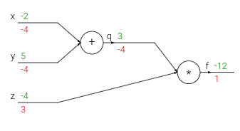
Backpropogation is a local process. Every gate in a circuit diagram gets some inputs and can right away compute two things: 1. its output value and 2. the local gradient of its output with respect to its inputs. The gates can do this completely independentlty without being aware of any of the details full circuit. Once the forward pass is over, during backprop the gate will eventually learn about the gradients of its output value on the final output of the entire circuit. And with the chain rule you take the gradient and multiply it by the gradient of its outputwith respect to its inputs.

This extra multiplication (for each input) due to the chain rule can turn a single and relatively useless gate into a cog of a complex circuit such as an entire neural network.

In the above example image, the intuition behind how backpropagation works using an example of a simple circuit with an add gate and a multiply gate.

The add gate receives inputs [-2, 5] and computes an output of 3. Since it’s performing addition, its local gradient for both inputs is +1.
The rest of the circuit computes the final value, which is -12.
During the backward pass, the add gate learns that the gradient for its output was -4. If we imagine the circuit as wanting to output a higher value, then the add gate “wants” its output to be lower due to the negative sign, with a force of 4.
To continue the chain rule and propagate gradients, the add gate multiplies the gradient (-4) to all of the local gradients for its inputs. This results in the gradient on both inputs (x and y) being -4.
This process has the desired effect: If the inputs were to decrease (in response to their negative gradients), the add gate’s output would decrease, causing the multiply gate’s output to increase.

Backpropogation can thus be thought of as gates communicating to each other (through the gradient signal) whether they want their outputs to increase or decrease (and how strongly), so as to make the final output value higher.

The derivative of the sigmoid function and its application in backpropagation for a neuron in a neural network.

The sigmoid function is defined as:

\[ \sigma(x) = \frac{1}{1 + e^{-x}} \]

The derivative of the sigmoid function with respect to its input x is derived as follows:

\[ \begin{align*} \sigma(x) &= \frac{1}{1 + e^{-x}} \\ \frac{d\sigma(x)}{dx} &= \frac{e^{-x}}{(1 + e^{-x})^2} \\ &= \frac{1}{1 + e^{-x}} \cdot \frac{e^{-x}}{1 + e^{-x}} \\ &= (1 - \sigma(x)) \cdot \sigma(x) \end{align*} \] This simplification of the gradient of the sigmoid function yields a straightforward expression: \((1 - \sigma(x)) \cdot \sigma(x)\).

In practical applications, this simplified expression is advantageous as it allows for efficient computation and reduces numerical issues.

The provided Python code demonstrates the backpropagation process for a neuron:

w = [2, -3, -3] # assume some random weights and data
x = [-1, -2]

# Forward pass
dot = w[0]*x[0] + w[1]*x[1] + w[2]
f = 1.0 / (1 + math.exp(-dot)) # Sigmoid function

# Backward pass through the neuron
# starting from end
ddot = (1 - f) * f # Gradient on dot variable, using the sigmoid gradient derivation
dx = [w[0] * ddot, w[1] * ddot] # Backprop into x
dw = [x[0] * ddot, x[1] * ddot, 1.0 * ddot] # Backprop into w
# We're done! We have the gradients on the inputs to the circuit

Backprop in practice: Staged computation

Suppose that we have a function of the form:

\[ f(x,y) = \frac{x + \sigma(y)}{\sigma(x) + (x + y)^2} \]

To be clear, this function is completely useless and it’s not clear why you would ever want to compute its gradient, except for the fact that it is a good example of backpropagation in practice

Here is the forward pass:

x = 3
y = -4

# forward pass
sigy = 1 / (1 + math.exp(-y))     # (1)
num = x + sigy                    # (2)
sigx = 1 / (1 + math.exp(-x))     # (3)
xy = x + y                        # (4) 
xy2 = xy**2                       # (5)
den = sigx + xy2                  # (6)
invden = 1/den                    # (7)
f = num * invden                  # (8)    

We have to compute gradients for sigy, num, sigx, xy, xy2, den, invden.

# backprop   f = num * invden 
dnum = invden # df/dnum = 1*invden + num*0 = invden
dinvden = num # df/dinvden

# backprop   invden = 1/den 
dden = dinvden * (-1/(den**2))
# self-learned-rule-of-thumb!
# for chain rule, instead of getting confused on 
# what to multiply because there are branches
# instead multiply the d of LHS, in above the example
# the function was
# invdev = 1/den
# we mul the dinvdev, which is dLHS.

# backprop den = sigx + xy2
dsigx = dden * 1
dxy2 = dden * 1

# backprop xy2 = xy**2
dxy = dxy2 * (2 * xy)

# backprop xy = x + y
dx = dxy * 1
dy = dxy * 1

# backprop sigx = 1 / (1 + math.exp(-x))
dx += dsigx * ((1-sigx) * sigx)         # Notice, +=, see notes below

# backprop num = x + sigy
dx += dnum * 1
dsigy = dnum * 1

# backprop sigy = 1 / (1 + math.exp(-y))
dy += dsigy * ((1-sigy) * sigy)

# Done!

Cache forward pass variables. To compute the backward pass it is very helpful to have some of the variables that were used in the forward pass. In practice you want to structure your code so that you cache these variables, and so that they are available during backpropagation. If this is too difficult, it is possible (but wasteful) to recompute them.

Gradients add up at forks. The forward expression involves the variables x,y multiple times, so when we perform backpropagation we must be careful to use += instead of = to accumulate the gradient on these variables (otherwise we would overwrite it). This follows the multivariable chain rule in Calculus, which states that if a variable branches out to different parts of the circuit, then the gradients that flow back to it will add.

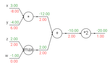
The add gate always takes the gradient on its output and distributes it equally to all of its inputs, regardless of what their values were during the forward pass. This follows from the fact that the local gradient for the add operation is simply +1.0, so the gradients on all inputs will exactly equal the gradients on the output because it will be multiplied by x1.0 (and remain unchanged). In the example circuit above, note that the + gate routed the gradient of 2.00 to both of its inputs, equally and unchanged. For this reason the add gate is also called gradient highway.¹

The max gate routes the gradient. Unlike the add gate which distributed the gradient unchanged to all its inputs, the max gate distributes the gradient (unchanged) to exactly one of its inputs (the input that had the highest value during the forward pass). This is because the local gradient for a max gate is 1.0 for the highest value, and 0.0 for all other values. In the example circuit above, the max operation routed the gradient of 2.00 to the z variable, which had a higher value than w, and the gradient on w remains zero.¹

The multiply gate is a little less easy to interpret. Its local gradients are the input values (except switched), and this is multiplied by the gradient on its output during the chain rule. In the example above, the gradient on x is -8.00, which is -4.00 x 2.00.¹

Unintuitive effects and their consequences.

Notice that if one of the inputs to the multiply gate is very small and the other is very big, then the multiply gate will do something slightly unintuitive: it will assign a relatively huge gradient to the small input and a tiny gradient to the large input. Note that in linear classifiers where the weights are dot producted \(w^T x_i\) (multiplied) with the inputs, this implies that the scale of the data has an effect on the magnitude of the gradient for the weights. For example, if you multiplied all input data examples \(x_i\) by 1000 during preprocessing, then the gradient on the weights will be 1000 times larger, and you’d have to lower the learning rate by that factor to compensate. This is why preprocessing matters a lot, sometimes in subtle ways! And having intuitive understanding for how the gradients flow can help you debug some of these cases.

Gradients for vectorized operations

Gradients for vectorized operations extend concepts to matrix and vector operations, requiring attention to dimensions and transpose operations.

Matrix-matrix multiplication presents a challenge: Forward pass:

W = np.random.randn(5, 10)
X = np.random.randn(10, 3)
D = W.dot(X)

Suppose we have the gradient on D:

dD = np.random.randn(*D.shape)  # same shape as D
dW = dD.dot(X.T)  # transpose of X
dX = W.T.dot(dD)

Tip: Utilize dimension analysis to derive gradient expressions. The resulting gradients must match the respective variable sizes. For instance, dW must match the size of W and depends on the matrix multiplication of X and dD.

Start with small, explicit examples to derive gradients manually, then generalize to efficient, vectorized forms. This approach aids understanding and application of vectorized expressions.

Gradient checking

TLDwrote; cs231n notes on gradient checking

Sources

Inspired by CS231n notes ↩ ↩² ↩³ ↩⁴
This blog is written as notes to this youtube lecture. ↩
CS231n Lecture on backprop can be found here. ↩

Table of contents