Parameter updates
Once the gradient is computed, it is then used to update the parameters. There are several approaches to perform the update.
Table of contents
- First order(SGD), momentum, nesterov momentum
- Per-parameter adaptive learning rates (Adagrad, RMSProp)
- Second order methods
- Sources
First order(SGD), momentum, nesterov momentum
Stochastic gradient descent
This is the vanilla update, the simplest form of update that changes the parameters along the negative gradient direction, as the gradient indicates the direction of increase, whereas we usually wish to minimize a loss. Assuming a vector of parameters x and the gradient dx, the simplest form of the update is as follows.
x += -learning_rate * dx # vanilla SGD update
Where learning_rate is the hyperparameter. In practice, we barely use this vanilla update because it is way too slow.
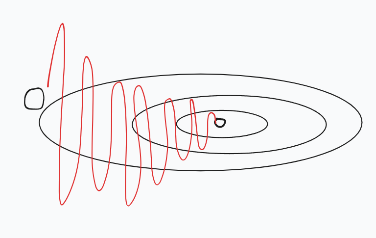
Consider a slope which is shallow horizontally and steep vertically. So with this approach, the gradients of the parameters would have high gradients vertically and small gradients horizontally, which then means the update would look like this.
Momentum Update
As the name suggests, this update applies momentum to the vanilla update.
Here is the formula.
V is equal to mu. times V Lr into gradient
X += V.
Where v is the momentum that we build along the process of training and mu is a hyperparameter that is used to decay the velocity, just like the friction decays the velocity of a ball rolling on the ground. This hyperparameter mu decays the velocity, and the process gradually converges.
This method overshoots but converges quickly compared to standard gradient descent.
Usually, the value of mu is set to 0.5 or 0.9, but sometimes it is annealed over time from 0.5 to 0.9.
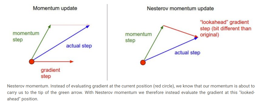
Nesterov Momentum (NAG)
Also called Nesterov accelerated gradient descent (NAG).
Nesterov momentum update modifies the ordinary momentum update with a technique “lookahead”.
Nesterov momentum is a slightly different version of momentum that has gained popularity. It enjoys stronger theoretical convergence guarantees for convex functions, and in practice, it also consistently works slightly better than standard momentum.
The core idea behind Nesterov momentum is that when the current parameter vector is at some position x, then looking at the momentum update above, we know that the momentum term alone (i.e. ignoring the second term with the gradient) is about to nudge the parameter vector by mu * v. Therefore, if we are about to compute the gradient, we can treat the future approximate position x + mu * v as a “lookahead” – this is a point in the vicinity of where we are soon going to end up. Hence, it makes sense to compute the gradient at x + mu * v instead of at the “old/stale” position x.
That is, in a slightly awkward notation, we would like to do the following:
x_ahead = x + mu * v
# evaluate dx_ahead (the gradient at x_ahead instead of at x)
v = mu * v - learning_rate * dx_ahead
x += v
However, in practice people prefer to express the update to look as similar to vanilla SGD or to the previous momentum update as possible. This is possible to achieve by manipulating the update above with a variable transform x_ahead = x + mu * v, and then expressing the update in terms of x_ahead instead of x. That is, the parameter vector we are actually storing is always the ahead version. The equations in terms of x_ahead (but renaming it back to x) then become:
v_prev = v # backup
v = mu * v - learning_rate * dx # velocity update stays the same
x += -mu * v_prev + (1 + mu) * v # position update changes form
Per-parameter adaptive learning rates (Adagrad, RMSProp)
Adagrad
We scale the gradient with an additional variable, cache.
cache += dx**2
x += -learning_rate * dx / sqrt(cache + 1e-7)
We are keeping the track of gradient for every single parameters. So this is often called per-parameter adaptive learning method. And then we divide the gradient element-wise with the square root of cache. This effectively changes the learning rate per parameter that is scaled dynamically based on their gradient.
TLDR;
- large gradient vertically
- are added up to cache
- this increase the cache size
- we end up dividing large number.
- We get smaller number in the update (the denominator is large)
- conclusion: The gradient updates are vertical. So, in this technique: the vertically updates are reduced and update look like this:
Problem with ADA grad: What happens as the step (epoch) size increases?
- the cache became larger and larger
- denominator becomes extremely big
- updates are reduced to almost None
But we don’t want this, in a deep neural network We want our optimization technique to keep shuffling the parameters untill we minimize the loss.
RMSProp (Gef. Hinton)
Instead of keeping the sum of square in cache, we define the cache so that it leaks and loses information so that it never grows too much big.
We set the decay hyperparameter– this way we are collecting the squares of gradient but slowly leaking it.
# ADAgrad
cache += dx**2
x += -learning_rate * dx / sqrt(cache + 1e-7)

# RMSProp
beta = 0.9 # leaking constant
cache = beta*cache + (1-beta)*(dx**2) # Notice removal of +=
x += -learning_rate * dx / sqrt(cache + 1e-7)

# I can see 2 kind of decay,
# - rapid decay on build up cache
# - slow decay on current grad parameters
Adagrad stops too quickly, but RMSProp continues.
Adam
This technique proposed update that looks a bit like RMSProp with Momentum update.
# recall the Momentum
v = mu * v - learning_rate * dx
x += v

# recall the RMSProp
beta = 0.9
cache = cache * beta + (1-beta) * (dx**2)
x += -learning_rate * dx / sqrt(cache + 1e-7)

# Adam
beta1 = 0.9 # decay hyparam for momentum
beta1 = 0.995 # decay hyparam for momentum

v = beta1 * v + (1-beta1) * dx
cache = cache * beta2 + (1-beta2) * (dx**2)
x += -learning_rate * v / sqrt(cache + 1e-7)

# commonly written as:
beta1 = 0.9
beta1 = 0.995

m = beta1 * m + (1-beta1) * dx
v = beta2 * v + (1-beta2) * (dx**2)
x += -learning_rate * m / sqrt(v + 1e-7)

### we often do

m /= (1-beta1)**t
v /= (1-beta2)**t
# > where t is the iteration in epoch
Dividing by (1 - beta1)^t and (1 - beta2)^t corrects these biases, especially at the beginning of training when t is small. This bias correction helps to make the estimates of m and v more accurate, leading to better optimization performance, particularly in the initial stages of training. ~ Karpathy.
AdamW
In AdamW, weight decay is incorporated directly into the update step for the parameters. Updated code for AdamW:
m = beta1 * m + (1-beta1) * dx
v = beta2 * v + (1-beta2) * (dx**2)
x += -learning_rate * (m / (sqrt(v) + 1e-7) + weight_decay * x)
AdamScheduleFree
By the time I was writing this blog, AdamScheduleFree was hot topic of research in meta
for each parameter group:
    retrieve beta1, beta2, learning rate (lr), weight decay, and epsilon (eps)

    for each parameter p in the group:
        retrieve or initialize m and v in state dictionary

        # Update m and v
        m = beta1 * m + (1 - beta1) * gradient
        v = beta2 * v + (1 - beta2) * (gradient ** 2)

        # Compute update
        update = -lr * m / (sqrt(v) + eps) + weight_decay * parameter

        # Update parameter
        parameter += update

        # Save updated m and v back to state
        save m and v in state dictionary
the state dictionary is used to store the momentum (m) and the exponentially weighted moving average of squared gradients (v) for each parameter. After each update step, these values are updated and stored back into the state dictionary for later use in subsequent optimization steps. The state dictionary is typically managed by the optimizer and is associated with each parameter being optimized.
Second order methods
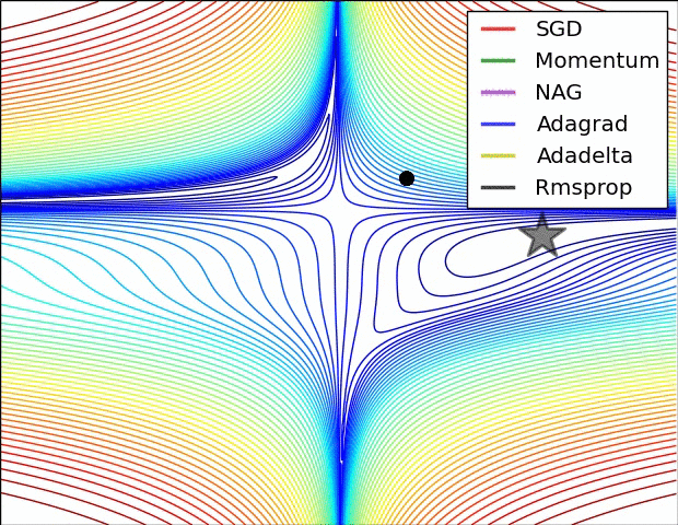
A second-order group of methods for optimization in deep learning is based on Newton’s method, which treats the following update. It uses a Hessian matrix, which is a matrix of second-order partial derivatives of the function. In particular, multiplying by the inverse Hessian leads to optimization taking more aggressive steps. So, if stochastic gradient descent techniques are used to find local minima one by one and piece by piece, the second-order method directly jumps to the local minimum of the surrounding area. However, the update above is impractical for most deep learning applications because computing such a large Hessian matrix and then inverting it is very costly, both in space and time. For instance, a neural network with 1 million parameters would have a Hessian matrix of size 1 million by 1 million, occupying approximately 3725 gigabytes of RAM. Hence, a large variety of approximation techniques have been developed that seek to approximate the inverse. Among these, the most popular is L-BFGS.
In practice, it is currently not common to see Lbfgs or similar second order methods applied to large scale deep learning and convolutional neural networks instead sgd variants based on nested momentum are more standard Because they’re simpler and scale more easily.
Sources
- Inspired from cs231n “Lecture 6: Neural Networks Part 3 / Intro to ConvNets”.
- cs231n Notes