Transformers
Back in 2017, the deep learning folks were trying to achieve state-of-the-art performance in sequence to sequence modeling. They used RNN’s like LSTM and GRU. The best performing model connects the encoder and decoder through an attention mechanism. Where the encoder is used to encode some sequence into rich embeddings and decoder decodes that embedding to different sequence. Example, language translation.
Table of contents
- Sequence to sequence modeling and limitations of RNNs
- Transformer
- Model Architecture
- Attention
- Feed Forward (Linear transformation)
- Input Embeddings (Vocab and Positional)
- Regularizations used in the paper
- Transformer Architectures
- Sources
Sequence to sequence modeling and limitations of RNNs
RNN had the vanishing gradient problem, models like LSTM and GRU emerged to tackle this problem but realized that altho the text may look better than rubbish, its still rubbish. It may look like English, but jumbled words and the sentence has no meaning.
- https://arxiv.org/pdf/1409.0473 (TLDR, first paper on using attention on RNN)
- https://arxiv.org/pdf/1601.06733 – This is a good paper on visualizing attention mechanism and using LSTM with Attention
They then tried to use attention mechanism with LSTM, Aligning the positions to steps in computation time, they generate a sequence of hidden states ht , as a function of the previous hidden state ht−1 and the input for position t. This inherently sequential nature precludes parallelization within training examples, which becomes critical at longer
sequence lengths, as memory constraints limit batching across examples. Recent work has achieved significant improvements in computational efficiency through factorization tricks and conditional computation, while also improving model performance in case of the latter. The fundamental constraint of sequential computation, however, remains.
RNN generates a sequence of hidden states ht, as a function of the previous hidden states ht-1 and the input for position t. This in a natural way, prevents the sequence to be trained parallelly, which becomes critical at longer sequence lengths, as memory constaints limit batching across examples. There are researches that had significant improvements in computational efficiency through factorization tricks and conditional computation, while also improving model performance. But the fundamental constraint of sequential computation still remains.
TLDR, one limitation is their computational complexity, especially with longer sequences, which can lead to slower training and inference times. They might struggle with capturing long-range dependencies in sequences.
Transformer
Transformer was the first model architecture which avoided RNN and instead relying entirly on an attention mechanism to draw global dependencies between input and output. Transformer allows for significantly more parallelization and thus requires less time to train.
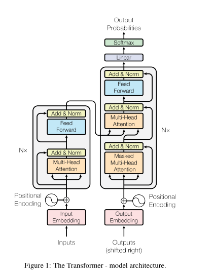
Model Architecture
The paper was for natural language translation and most competitive neural sequence transduction model have an encoder-decoder structure, so the transformer proposed is also an encoder-decoder transformer. Where the encoder took sequence x (1->n) and generates continuous representation z (1->n). Given z, the decoder then generates an output sequence one element at a time. At each step the model is auto-regressive. Consuming the previously generated symbols as additinal input when generating the next.
Attention
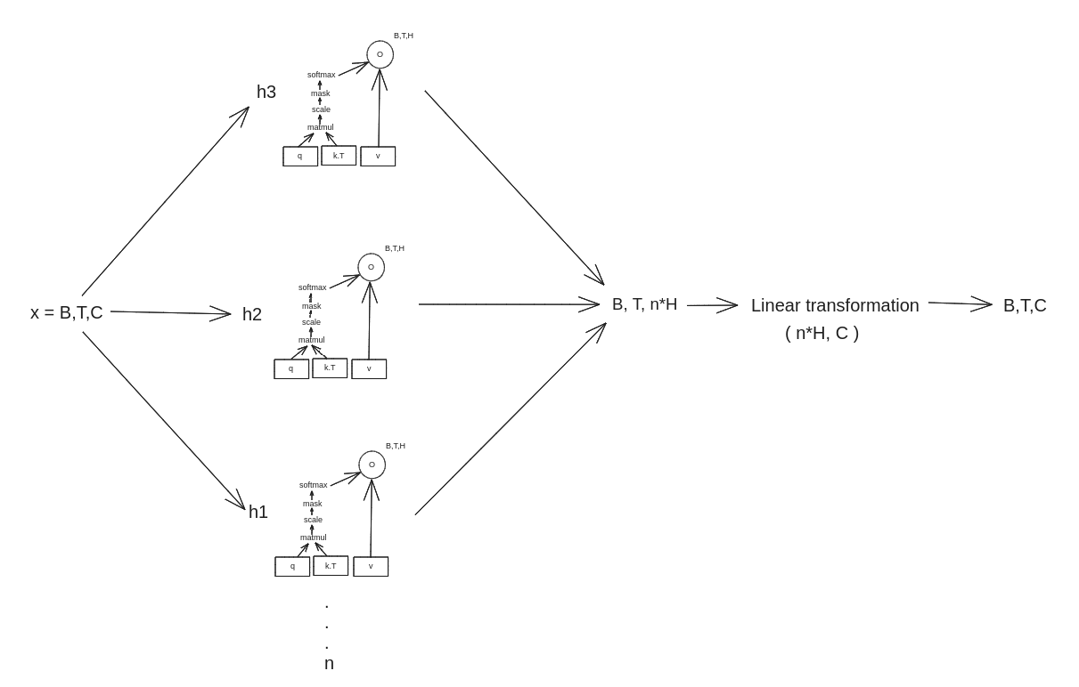
Understanding the attention is the core of transformer. Attention can be defined as mapping a query and a set of key-value pairs to an output, where the query, key, values and output are all vectors.
Each vector is derived from the input X. In relatable words, to interpret this, think you have
- a query matrix as a question or prompt (all latent factors, you know nothing about what kind of query is present),
- and the key as a set of potential answers or relevant information.
- By multiplying the query with the transpose of the key, you’re essentially comparing the question with each potential answer to determine their similarity/relevance.
- you get the attention score, (typically scaled and then normalized using softmax) scale? why? because big numbers == more computation.
- this normalized attention distribution will then guide the model (talking about optimization process aka backprop) on how much weight to assign to each value when computing weighted sum, which represents the attended information or the answer to the query.
Types of attention function
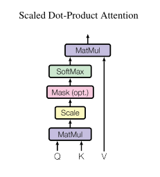
The two most commonly used attention functions are additive attention, and dot-product attention. Additive attention computes the compatibility function using a feed forward network with a single hidden layer. Both achieves the same but the dot-product attention is much faster and more space-efficient in practice, since it can be implemented using highly optimized matrix multiplication code.
After the matrix multiplication, we scale the output by 1/(Dk)**0.5. Where, Dk is the dimension of keys and queries. After that we apply softmax to obtain weights on the values.
Why scaling
While for the small value of Dk, additive function outperforms the dot-product attention without scaling for larger value of Dk. This is because, when the value of Dk is small, softmax receives bigger input which tends the softmax to create the probability distribution more easily. But, as we scale the dimension of head, i.e head_size (Dk) the input to softmax gets smaller and its hard for softmax to distribute the probability. To counteract this effect, we scale the dot product by 1/(Dk)**0.5.
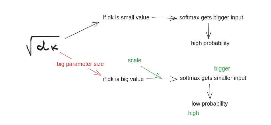
Therefore, we use scaled dot-product attention rather than additive attention without scaling.
Multihead attention
Instead of performing a single attention function with d dimension– d keys, queries and values, it is beneficial to linearly project the queries, keys and values n times with different. We then perform the attention function in parallel, yielding n times head_size output values. These are then concatenated and then have a linear transformation.
Auto-regression mask for self-attention Head (Masked-attention)
Recall this attention mechanism, but what is the mask?
We create a triangular matrix, 0’s on the top right and 1’s on the bottom left.
>>> import torch
>>> torch.tril(torch.ones((4,4)))
tensor([[1., 0., 0., 0.],
        [1., 1., 0., 0.],
        [1., 1., 1., 0.],
        [1., 1., 1., 1.]])
take another matrix
>>> torch.randn(4,4)
tensor([[ 0.8350,  1.4479, -2.2848, -1.5227],  # <- Sequence 1 acts
        [-0.8851, -0.4905, -1.1630, -1.0715],  # <- Sequence 2 ''
        [ 1.0836, -1.5426,  1.9595, -1.3338],  # <- Sequence 3 ''
        [-0.3320,  0.5324,  0.2499, -0.5427]]) # <- Sequence 4 ''
Now if we have matrix multiplication, the 0’s effectively cancels the future occuring numbers.
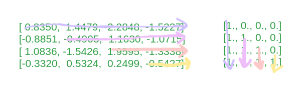
We can improve this, instead of zeros in the mask matrix, if we replace them with -inf it will help Softmax. Replacing zeros with -inf in the triangular matrix masks future tokens, ensuring the model only attends to past and present tokens during self-attention by setting future attention scores to effectively zero.
>>> torch.tensor(float('-inf')).exp()
tensor(0.)
>>> torch.tensor(0).exp()
tensor(1.)
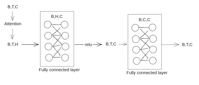
Feed Forward (Linear transformation)
In addition to attention sub-layers, each of the layers in encoder and decoder contains a fully connected feed-forward network, which is applied to each position separately and identically. This consists of two linear transformations with a ReLU activation in between.
FF(x) = [W1*x + B1] -> [relu] -> [h -> W2*h + B2]
Input Embeddings (Vocab and Positional)
Purpose. Since the model has no conv or recurrent network, in order to make the use of the order of the sequence, we must inject some information about the relative or absolute position of the token in sequence. Therefore, in addition to the classic vocab embedding (embedding for each token) we also add embeddings for each position in the sequence. The positional embeddings have the same dimension as the embeddings, so that the two can be summed.
Choice. It is possible to start with a Fixed positional embedding or learned positional encoding, it is mentioned in the research paper that they found the two version produced nearly identical results. Hence, they choose the sine version (fixed) because it may allow the model to extrapolate to sequence lengths longer than the ones encountered during training. Fixed positional encodings are pre-defined functions that map each position in the sequence to a fixed vector representation. Useful resource.
read TransformerXL paper.
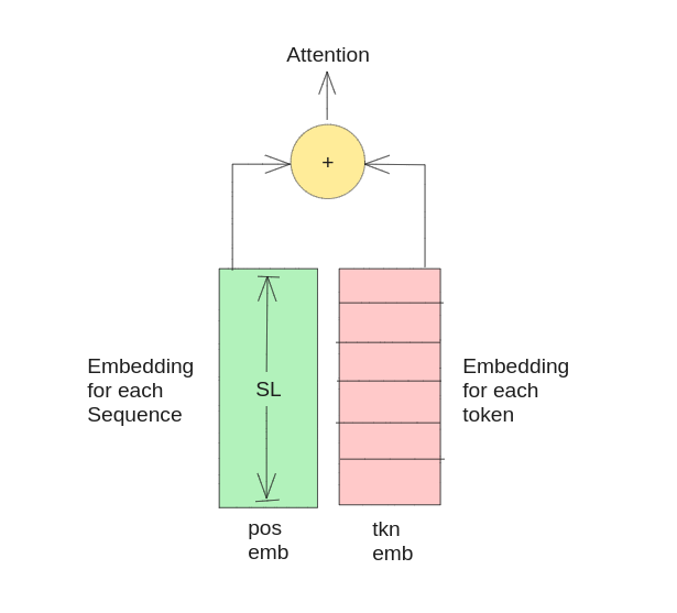
Comparison. both versions produced nearly identical results, suggesting that the choice of positional encoding method did not significantly impact model performance. Ultimately, the authors opted for the sinusoidal positional encodings due to their potential for extrapolating to longer sequence lengths beyond those seen in training data.
Regularizations used in the paper
- Residual Dropout: dropout to the output of each sublayer before it is added to the sublayer input and normalized. Dropout is also applied to the sum of embeddings and positional embeddings in both encoder and decoder stack. (p=0.1)
- Label Smoothing: instead of one hot encoded labels, smoothing the layers. high-level example:
0,1,0 -> 0.1, 0.8, 0.1.
Transformer Architectures
Encoder-Decoder
Used for sequence to sequence task like translation, summarization. Encoder process the input sequence, decoder with masked-self-attention, cross-attention over encoder output and feed forward sub layers. Generates output sequence autogressively.
Here is the intution, the encoder creates feature rich representation of the input sequence, the decoder then uses the memory (i.e, key-value) of the encoder to generate output autoregressively. But the decoder also has the feature rich representation of inputs (i.e, query).
The using of encoder’s attention in decoder is called cross-attention. (encoder: key-value –> decoder: query)
Encoder only
Used for task like text classification, feature extraction, pretrained representations, document embeddings, transfer learnings.
basically creating feature rich embeddings for given sequence. The embedding then can be used to different tasks mentioned above.
Decoder only
Used for language modeling, text generation tasks. Decoder components are masked self-attention and feed-forward layers, no encoder, no cross attention. Autoregressive in nature (due to attn-mask).