CNNs
This is a quick skim notes for CS231n Introduction to CNN lecture 7, I used slides from this lecture to create notes and this is NOT an attempt to replicate notes by cs231n, its already the best notes on CNNs out there.
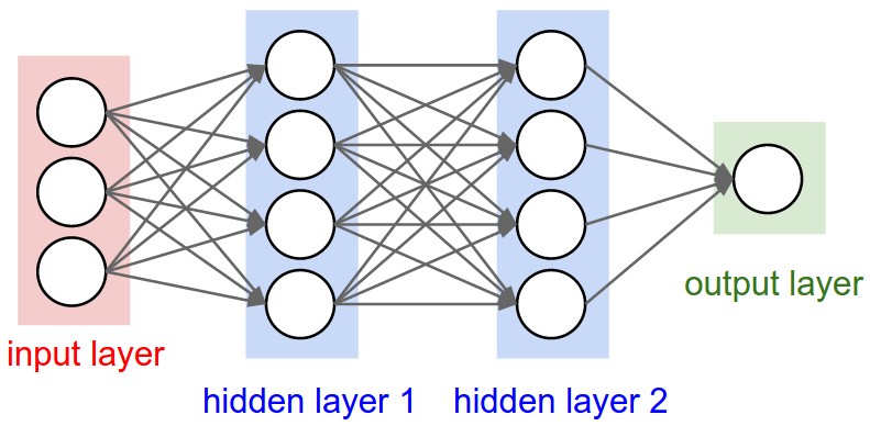
CNNs are similar to ordinary neural networks, they have trainable weights and bias, receives input, bunch of trainable layers followed with non-linearity. Each layer is completely differentiable, means they can learn. At the end an output layer predicting classes or so.
So what changes? ConvNet architecture make the explicit assumption that the inputs are image which allows us to encode certain properties into the architecture. These then make the forward function more efficient to implement and vastly reduce the amount of parameter in the network.
Why can’t regular NNs don’t scale to images?
Consider an image from CIFAR-10 dataset, size 32x32x3, input neurons would be 32x32x3 = 3072 weights. Good? Now consider an image 200x200x3 image, 120,000 weights in the first layer, moreover we would almost certainly want to have several such neurons, so the parameters would add up quickly. Clearly, this full connectivity is wasteful and the huge number of parameters would quickly lead to overfitting.
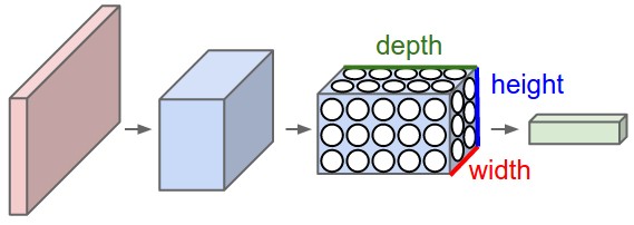
3D volumes of neurons
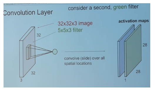
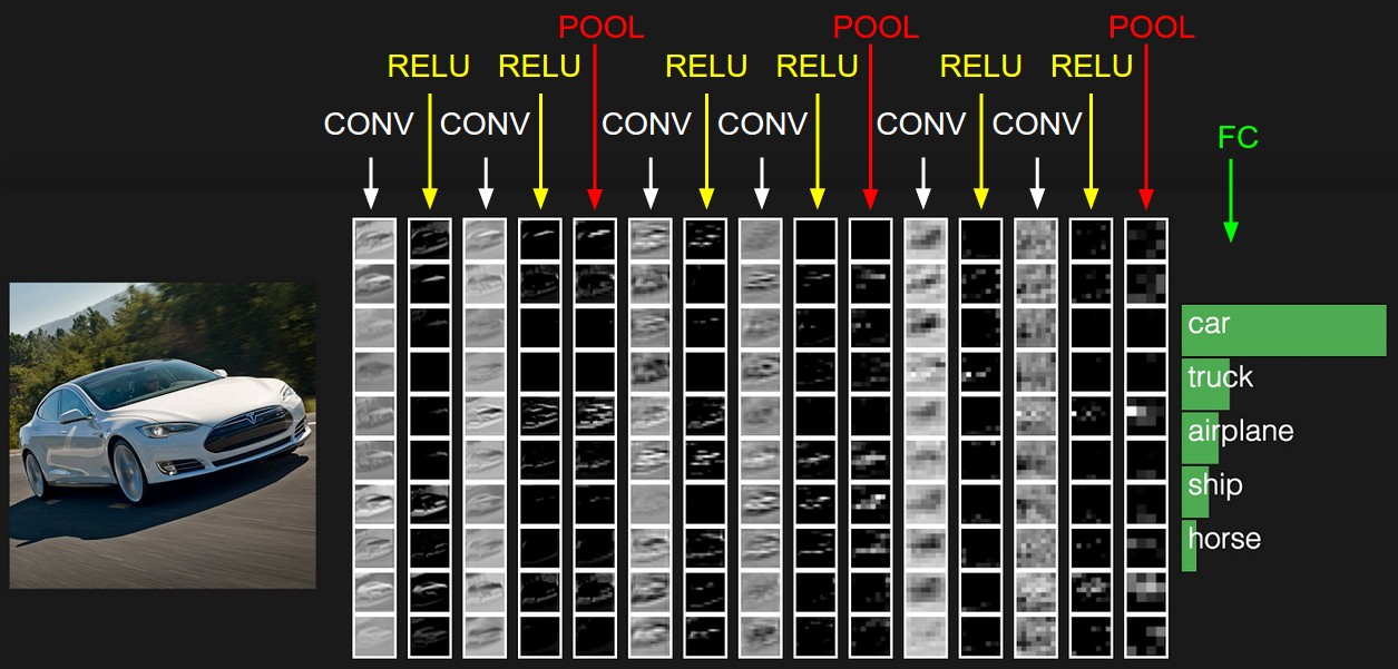
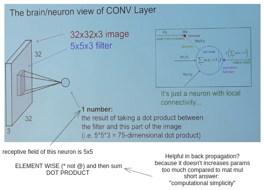
CNN’s take the advantage of the fact that the input are images and use the architecture in a more sensible way. In particular, unlike the regular neural networks the layer of convolution net have neurons arranged in three dimensions: Height, width and depth. The depth here is not the depth of the whole neural net. But instead, it’s the depth of trainable weights. A good visualization:
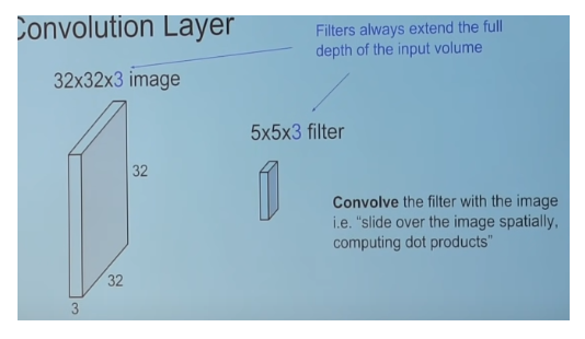
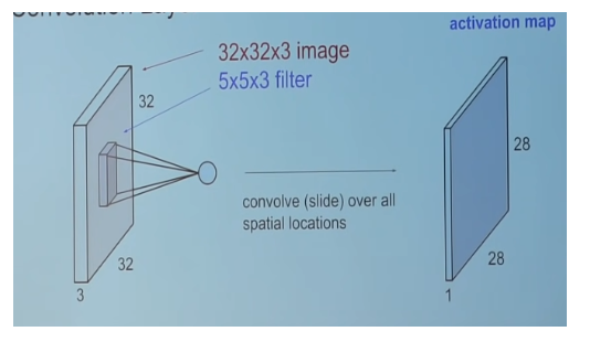
Convolve
Filters, also called kernels, are small (typically 3x3 or 5x5) used to slide over the image spatially, computing dot products. The filters also have depth, eg. 3x3x96 here 96 is depth of the kernel. The depth of kernel should be equal to the depth of the input. If the input is 32x32x3 image, where 3 is ~RGB. then kernel would have depth 3 (3x3x3 or 5x5x3).
in the above case, spatial dimension is the 32x32 (height and width of input).
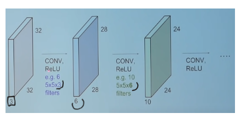
An overview of the ConvNet architecture
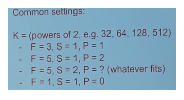
How do we know, the size of the output after convolution?
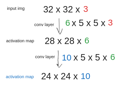
(N-F)/S + 1, where N is the number if input dimension, F is the kernel dimension. S is stride.
Oh yes, what is Stride?
Kernels slide through the input layer, Stride refers to number of pixels the filter mover over the input image during convolution (see some gifs)
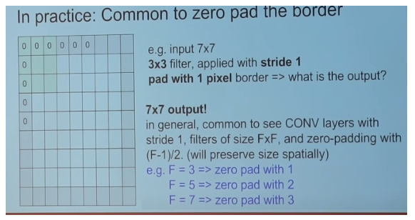
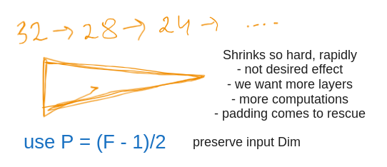
Padding
In practice, it is common to pad the input image with 0s around the edges.
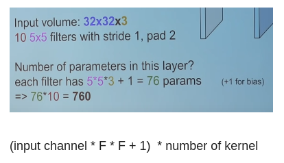
math time, calculate how many trainable params
we can also have 1x1 Kernels
Summary 1: Convolution Layer
- Accepts input of shape W, H, D
- Requires hyperparameters
- Number of Kernels– N
- Kernel dim– F
- Stride– S
- Padding– P
The brain/neuron view of CONV layer
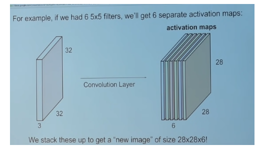
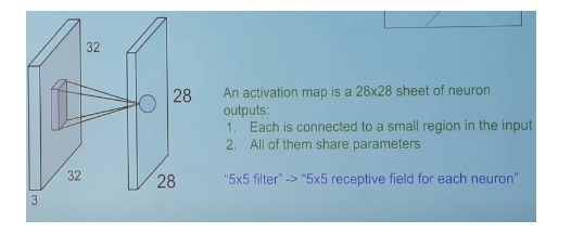
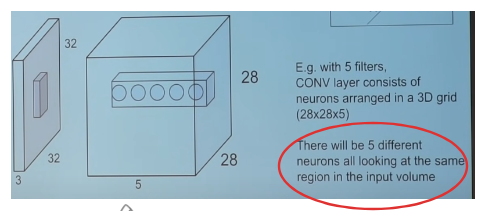
Recall how the activation map depth is equal to the number of kernels.
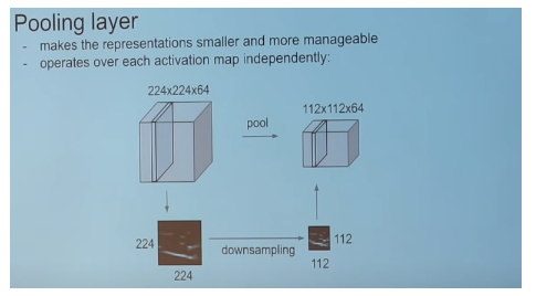
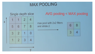
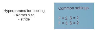
Pooling Layer
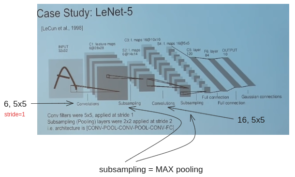
Case Study
LeNet-5
AlexNet
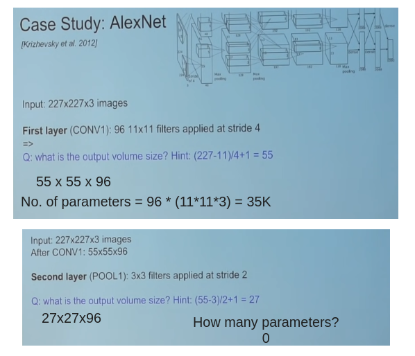
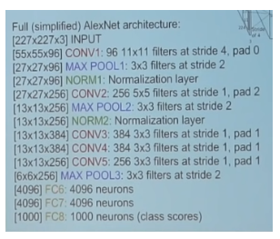
Architecture of AlexNet: C = Conv, P = Pool, O = Output layer
[C-P-C-P-C-C-C-P-FC-FC-O-Softmax]
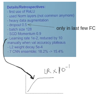
some details:
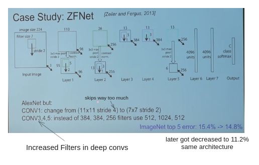
ZFNet
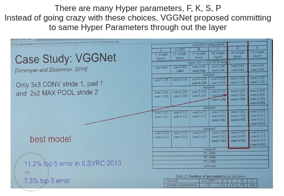
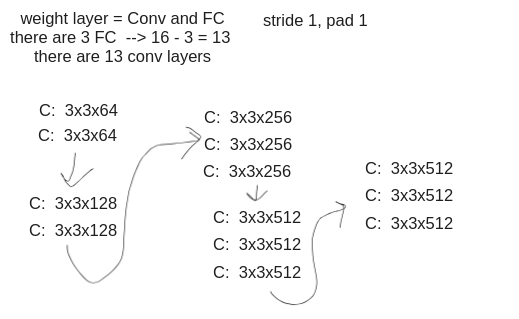
VGGNet
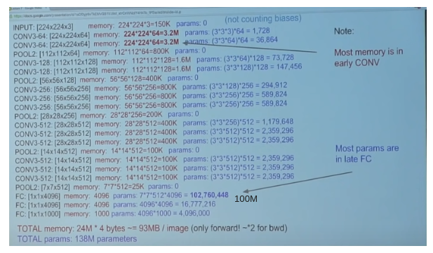
Memory footprint of VGGNet shows,
- Most memory is in early CONV layer (3M)
- Most Parameters are in late FC layers (10M)
- 93MB/image in forward pass alone
Average Pooling Layer replaces FC layer in the end
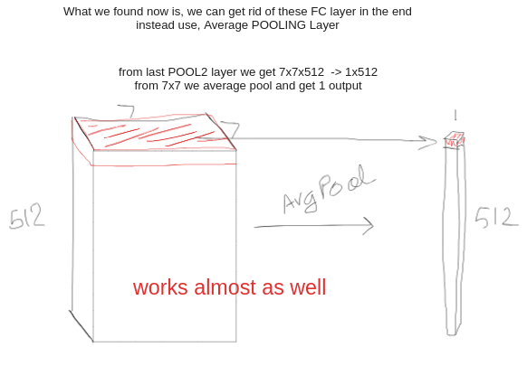
The example is from the FC layer of VGG net, the last POOL2 output is of shape: 7x7x512, where 7x7 are spatial dim and 512 is depth/volume. each 7x7 is averaged pool to 1. reducing the size quite a lot.
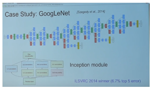
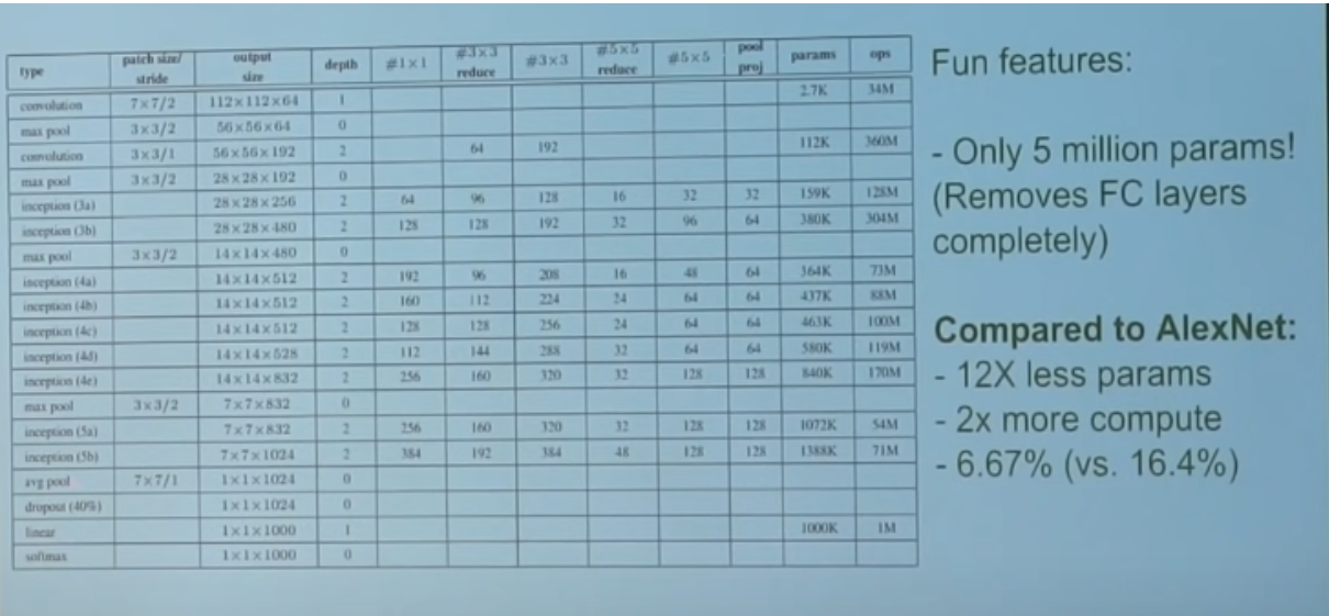
GoogLeNet (introduced inception)
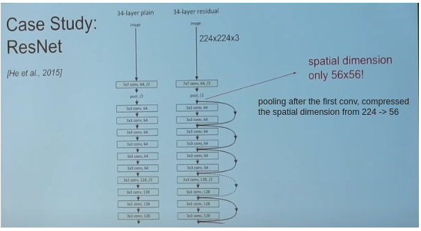
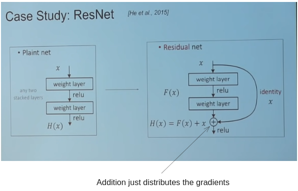
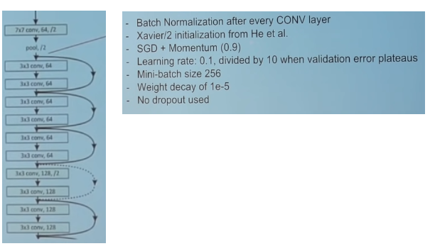
ResNet
In 2015, ResNet won 1st place in many competition at the same time. GoogleNet was 22 layers, introduced resnet was 152 layers.
So increasing layers == win?
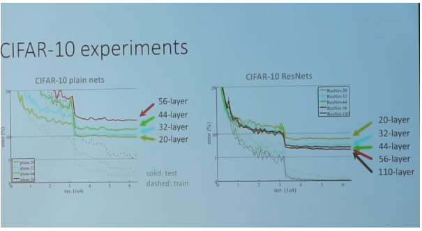
ResNet took, 2-3 weeks of training on 8 GPU, but at runtime, its faster than VGGNet, even though it has 8x more layers.
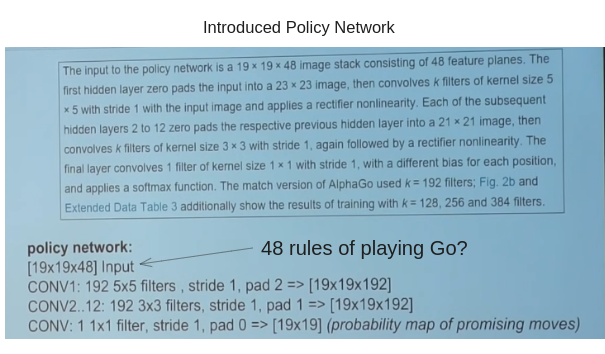
AlphaGo (policy network?)
Playing Go (harder than chess) using CNNs? The 48 rules of playing Go embedding into the image’s channel?
Summary 2: Trends
- ConvNets Stack Conv, pool, FC layers
- Smaller filters and deep architecture
- get rid of Pool/FC layers (just convs)
- Treads toward stride-convs only layer, where you try to reduce image dimension (not depth) using convs instead of using pooling layer.
- ResNet/GoogleNet challenge this paradigm