Interpretable Features from Neural Networks
I watched a podcast of Jensen and Ilya, in which Ilya talked about how multimodality enables neural networks to learn more features than just a single modality. For example, large language models like GPT-4, without vision, can recognize that the color pink is close to red, but they can’t explain why, because they haven’t seen a single pixel. Multimodality combines image and text, both trained in a unified way. And GPT-4 with vision can tell exactly which pixel is red and why. To achieve intelligence smarter than human-level intelligence, we will definitely need multimodality, because our world is very visual, and neural networks can learn a lot from it.
I can relate his thoughts from this video “Why Humans are intelligent?”:
1) Communication, they can pass their knowledge to future generation whereas cats and dogs can't.
2) They can interact with the surrounding world/environment.
3) eye sight.
So, I shifted my gears from architectural improvements (I will come back to it, but when time comes) to multimodality.
The first thing that came to mind was:
> revise CNNs
  > created a blog post on it.
> There must be something good in fast.ai course that I left unfinished after NLP.
  > found it, UNet!
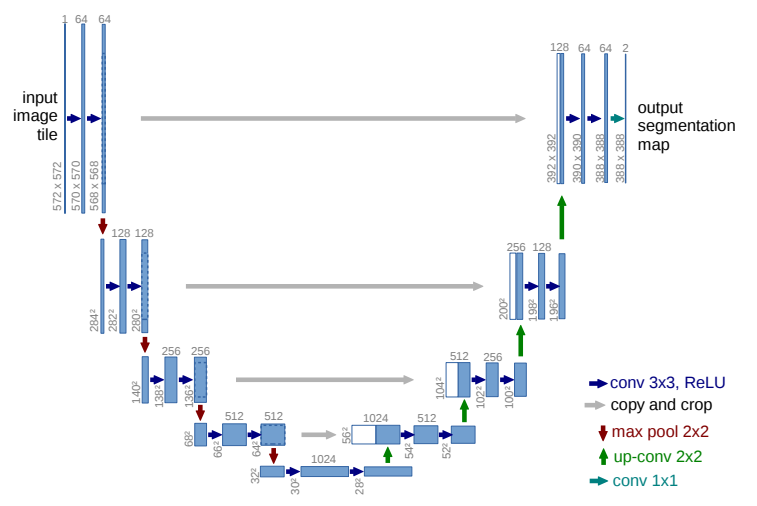
What is U-Net?
U-Net came out before ResNet and was originally focused on medical applications but it has now revolutionized all kinds of generative vision models. This is what I learned. The basic idea is to start with pretrained model (like alexnet or VGG?) and instead of predicting labels, cut the head and add custom head that “reconstructs the input image”.
How can we do that? The convolution layer is used to reduce the special dimension and increase the features (depth)?
The basic idea is, once you have a feature map (activations) say 7x7, what if you replace each element of the 7x7 with 2x2 matrix? the result would be 14x14. This process is called nearest neighbour interpolation (NNI). In which every pixel is replaced by a grid of same pixel. Another approach is called transpose convolution. In which, first we pad each of the input pixel with 0s and then use a kernel (3x3 common to use) with stride 1. This results in the same effect. [Check it with this formula (L-K)/S + 1]. Here is a good visulization.
The difference between Nearest neighbour interpolation and Transpose convolutions.
Nearest neighbour interpolation is fast and no learnable parameters, whereas Transpose kernel has learnable parameters (kernel) but slow.
I was trying to solve a competetion by comma.ai, in which we have compress a numpy vectors losslessly. And I found out that the SOTA open source self-driving model uses Nearest neighbour interpolation. Whereas, generative ai, where we use transpose convs in generative ai (I assume, haven’t looked into GANs, VAEs, diffusion etc. YET).
The architecture of U-Net.
UNet is an encoder decoder structure, the Encoder encodes the input image to features by using conv-pool-conv-pool. Later the Decoder decodes the activation map using transpose convs (up): up-conv-up-conv. The game changer is the residual connections.
Residual connections in a nutshell: Instead of learning the full output, the network learns the “residuals”, or the difference, between the input and the desired output. This is achieved by adding the input to the output, effectively “jumping over” one or more layers. This allows the network to focus on learning the residual, or the error, rather than the full output.
It’s easier for the network to learn the residual between the input and output, rather than learning the full output from scratch. (Kaiming He et al. 2016).
Next, new paper on interpretability of LLMs by anthropic.com
> my thoughts. They used sparse autoencoder,
  a kind of dictionary learning to extract the features of their production
  level model Claude Sonnet.
  > what the heck is dictionary learning and Sparse autoencoder?
> I researched and found a paper/notes
  > https://web.stanford.edu/class/cs294a/sparseAutoencoder.pdf
Dictionary learning
A technique that involves learning basic functions (features) that can be used to represent input data efficiently.
Deep learning approach is called autoencoders
An autoencoder neural network is an unsupervised learning that applies backpropagation, setting the target equal to the input. In other words, the autoencoder tries to learn a function aims to reconstruct the original input. This function can be then used to visualize features of the input data.
As a concrete example, suppose the inputs x are the pixel intensity values from a 10×10 image (100 pixels) so for our first layer the input features is n = 100, and there are 50 hidden units in layer L2. And the output would be 100 same as the input. Since there is only 50 hidden units, the network is forced to learn a compressed representation of the input.
10x10 -> 1,100 -> 100x50 -> 50x100 -> 1,100 -> 10x10
Let’s say, if the input is a completely random noise, then it would be hard and very difficult for this compression task. But if there is a structure in the data, Then this algorithm will be able to discover some of those correlation. In fact, this simple autoencoder often ends up learning a low-dimensional representation very similar to PCA’s.
If we impose a contraint other than ‘compression’, say opposite, greater (perhaps even greater than the number of inputs pixels) we can still discover interesting patterns. This is called the sparsity constraint on the hidden units. This will cause most of the neurons in the large activations to say zero or near zero (in-active) only firing few neurons for special data – Sparse Autoencoder!!!
Consider a hidden layer in a neural network where we have a sparse autoencoder. In a typical sparse autoencoder, we want most of the neurons to be inactive (close to zero) and only a few to be active for any given input.
Imagine you have an activation vector A from a hidden layer with 10 neurons for a particular input:
# say our activations: the result of 1,100 * 100x50 = 1x50  is:
a = torch.randn((1,50))
For this vector, suppose we want only 10% of the neurons to be active on average (making 90% close to zero or inactive and 10% close to 1, active). To enforce this sparisity, we need a way to measure how far the input data distrubution is from our output distribution.
KL divergence does that.
KL divergence is a measure of how one distribution differs from a another distribution.
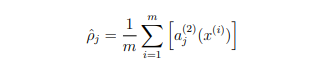
we want the constrain this "rho_hat" to something like 0.05. Sparse.
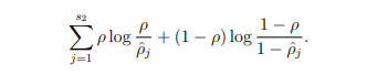
s2 is the number of neuron in the hidden layer, p (rho) is the sparisity parameter (0.05 what we decided), in other words we would like the average activations of each hidden neurons to have to be close to p "sparsity parameter". This is the KL divergence, which tells us how distance is the distribution of activations (rho_hat) from what we want (rho).
We can use KL divergence as our criterion (loss function), infact this is very close to cross-entropy loss.
the difference between cross-entropy loss and KL divergence is, the cross-entropy loss calculates the distance between predictions and labels. Whereas, KL divergence calculates the difference between two distance distributions.
To incorporate the KL-divergence term into the derivative calculation, we only need a small change, in addition to gradient, we also accumulate the average of activations on all training set, before backprop. and now in the backprop we can add the sparsity penalty as well as the weight decay.
# assuming we have
avg_z # average of all activation, basically acts.mean(0)
rho_t # sparsity parameter, same size avg_z but "full_like"!

# restoration loss
r_loss = criterion(_x, x) # where _x is the reconstructed x
# kl divergence
kl_d = rho_t * torch.log(rho_t/avg_z) + (1 - rho_t) * torch.log((1-rho_t) / (1-avg_z))
# sparsity penalty
sp = beta + torch.sum(kl_d) # where 'beta' is the strength of penalty
loss = r_loss + sp
Here is my Sparse autoencoder implementation.
there are 2 versions, 2nd is the sparse, 3rd is compressed
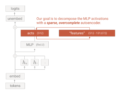
Back to Antropic’s paper
Antropic team, grabbed a layer’s activation of Claude 3 Sonnet from somewhere in “middle” 1 and trained their sparse autoencoder in it.
# implementation
encoder = Linear(input_dim, hidden_dim)
decoder = Linear(hidden_dim, input_dim)

# x is the input
encoded = torch.relu(encoder(x))
decoded = decoder(encoded)

# loss
r_loss = torch.mean((x - x_hat) ** 2) # MSE
sp = torch.sum(torch.abs(encoded), 1).mean()

loss = r_loss + _lambda + sp
Notice this:
- Antropic used L1 penalty directly on acts
-
Stanford notes used KL divergence to penalize deviations
- Antropic directly used magnitude of activations
- Stanford ensured to use averaged activations
Features
- just skim over these: long story short, LLMs activations if touched every RL saftey breaks. LLMs follow sycophancy, which means the tendency of models to provide responses that match user beliefs or desires rather than truthful ones. The models are not truthful.
Next steps?
- multimodality is the key to intelligence
- speech recognition and synthesis
- notes and my notion
References
- every other source is provided directly in the hyperlink.